End-to-end SAR flood mapping pipeline
From raw SAR to a flood map, in your browser.
Code cells are interactive examples: click Run to reveal the expected output. Full reproduction requires a configured local Jupyter/WSL environment, SNAP GPT, dataset paths, credentials, CUDA/onnxruntime, and the model checkpoint.
01 · SAR Acquisition
Sentinel-1 C-band · GRD · IW · VV+VH · ~10 m
Optical sensors were blind here — total cloud. So how does radar see flooding through cloud, and even at night?
# Copernicus Data Space Ecosystem (CDSE) OData search
# 3 acquisitions needed: pre-event 1, pre-event 2, post-event

from sentinelsat import SentinelAPI
api = SentinelAPI('user', 'pass',
                  'https://dataspace.copernicus.eu/odata/v1')

footprint = 'POLYGON((95.2 5.4, 95.5 5.4, 95.5 5.6, 95.2 5.6, 95.2 5.4))'

products = api.query(footprint,
    date=('20241201', '20250115'),
    platformname='Sentinel-1',
    producttype='GRD',
    sensoroperationalmode='IW')

print(f"Found {len(products)} products")
api.download_all(products)
Found 6 products matching AOI + date range
Selected 3 GRD products for the teaching workflow:
Downloading S1A_IW_GRDH_1SDV_20241210T112358_..._039E_010D_84F5.SAFE.zip
Downloading S1A_IW_GRDH_1SDV_20241222T112358_..._039E_010D_9A21.SAFE.zip
Downloading S1A_IW_GRDH_1SDV_20250103T112357_..._039E_010D_AF4D.SAFE.zip
Done · 3 files queued for preprocessing
Ask anything about this step — or start with:
one shared thread with the floating tutor · + new · history above
02 · GRD Preprocessing
SNAP GPT · 10-operator XML graph → calibrated σ0 GeoTIFF
Ten operators turn raw radar into a clean image. What has to be true before two dates can be compared pixel-for-pixel?
# SNAP Graph Processing Tool — runs the full chain as one XML
# Pipeline: Read → Orbit → Subset → ThermalNoise → BorderNoise
#         → LandSeaMask → Calibration(σ0) → SpeckleFilter(LeeSigma)
#         → TerrainCorrection → Write(GeoTIFF)

$ gpt grd_preprocessing_srtm.xml \
    -PinputFile=S1A_IW_GRDH_..._post.SAFE \
    -PgeoRegion="POLYGON((95.2 5.4, 95.5 5.4, 95.5 5.6, 95.2 5.6, 95.2 5.4))" \
    -PoutputFile=sigma0_post_vv_vh.tif
Read               : S1A_IW_GRDH_..._post.SAFE
Apply-Orbit-File   : precise orbit ephemeris attached
Subset             : AOI clipped to 34.2 km × 28.7 km
ThermalNoiseRemoval → Calibration (σ0) → Speckle (Lee Sigma 3×3)
Terrain-Correction : 10.0 m pixel spacing · EPSG:4326
Write              : sigma0_post_vv_vh.tif

Done in 04:18 · 2 bands written: Sigma0_VV, Sigma0_VH
# Two XML variants — only the DEM source differs:

# Variant A: auto-download SRTM 1-arc-second
<demName>SRTM 1Sec HGT</demName>

# Variant B: user-supplied external DEM (e.g. Copernicus GLO-30)
<demName>External DEM</demName>
<externalDEMFile>${externalDEMFile}</externalDEMFile>

# Shared across both:
Calibration  → outputSigmaBand = true    # linear σ0
SpeckleFilter→ filter = "Lee Sigma", 3×3  # mild smoothing
TerrainCorr  → pixelSpacing = 10.0 m     # output resolution
03 · Tiling & Normalisation
224×224 patches · clamp + z-score · the preprocessing knob
Same model, same data — only the clamp changed, and the flood vanished. What is the clamp throwing away?
import numpy as np

# KuroSiwo training statistics
CLAMP  = 0.15       # upper tail cutoff
VV_MEAN, VV_STD = 0.0953, 0.0427
VH_MEAN, VH_STD = 0.0264, 0.0215

def normalise(sigma0, pol='vv', clamp=CLAMP):
    mean, std = (VV_MEAN, VV_STD) if pol == 'vv' else (VH_MEAN, VH_STD)
    x = np.clip(sigma0, 0, clamp)    # clamp upper tail
    x = np.nan_to_num(x, nan=clamp)  # NaN → clamp ceiling
    return (x - mean) / std           # z-score

# The clamp ceiling controls everything:
# Banda Aceh VH peak σ0 ≈ 0.40  (training mean: 0.026)
# clamp 0.15 → truncates flood signal to nothing
# clamp 0.30 → recovers flood signature
normalise(post_vh, pol='vh')  →  float32(224, 224), z-scored

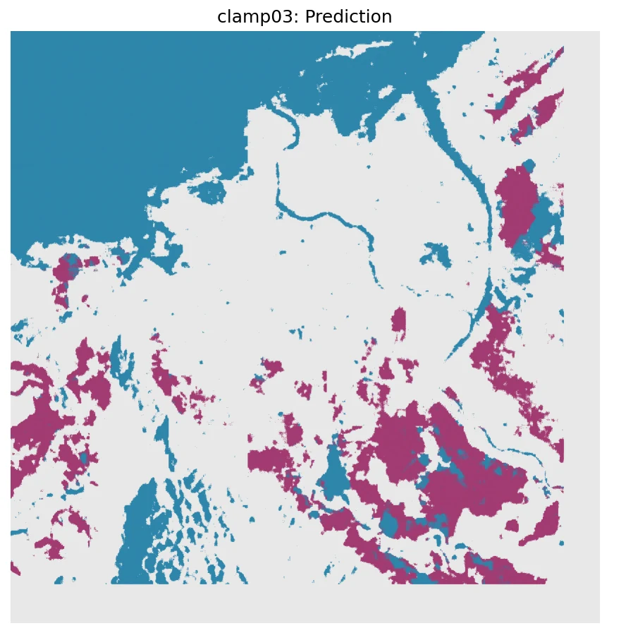
Banda Aceh post-event VH σ0 peaks ~0.40 (flood scatters bright) —
but the training mean is 0.026, so the model expects a much dimmer tail.
  clamp 0.15 : every value above 0.15 is pinned to the ceiling →
               the bright flood tail is flattened away before the model sees it
  clamp 0.30 : the ceiling clears the flood tail → the signal survives
Same pixels in — only the ceiling differs.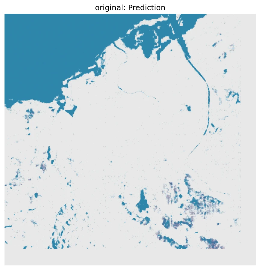
# Model expects: [pre2_vv, pre2_vh, pre1_vv, pre1_vh, post_vv, post_vh]
# Each channel: 224×224 float32, z-scored

tensor = np.stack([
    normalise(pre2_vv, 'vv'), normalise(pre2_vh, 'vh'),
    normalise(pre1_vv, 'vv'), normalise(pre1_vh, 'vh'),
    normalise(post_vv, 'vv'), normalise(post_vh, 'vh'),
])  # shape: (6, 224, 224), dtype: float32

tensor.tofile('input.bin')  # 6 × 224 × 224 × 4 = 1,204,224 bytes
tensor.shape  = (6, 224, 224)
tensor.dtype  = float32
channels      = [pre2_vv, pre2_vh, pre1_vv, pre1_vh, post_vv, post_vh]
per-channel z-score (clamp 0.15) → mean ≈ 0.00 · std ≈ 1.00
wrote input.bin · 1,204,224 bytes
What one 224² tile is made of.
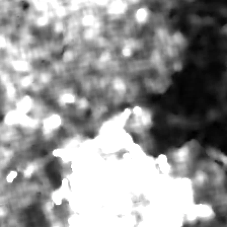
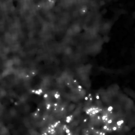
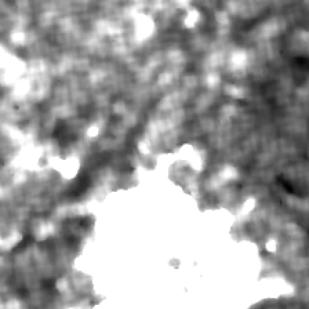
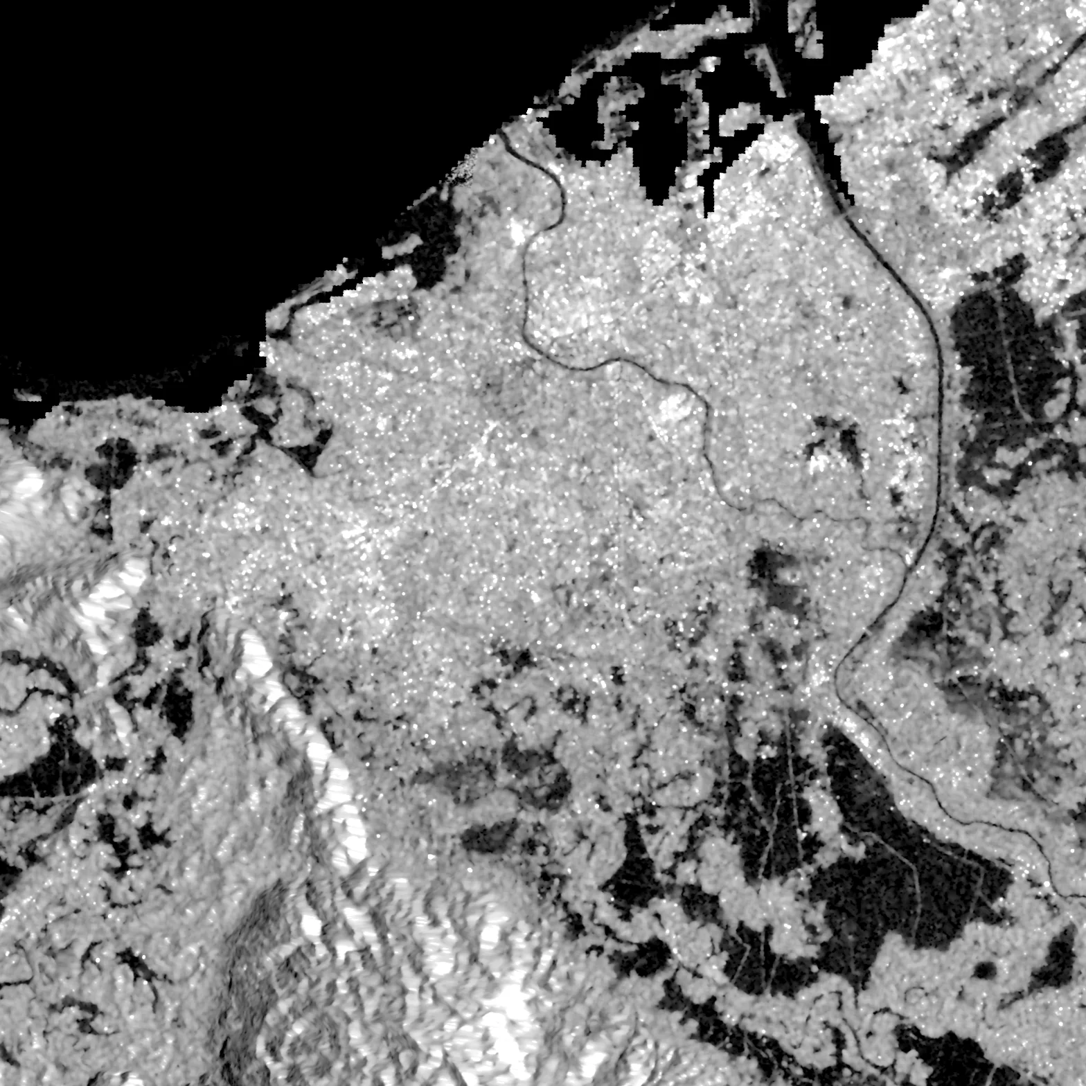
Each KuroSiwo-format tile stacks 6 bands — VV + VH at three acquisition times: pre-event 1 (21 Oct, baseline), pre-event 2 (2 Nov, approach) and co-event (26 Nov, the flood). Here are the three VV composites of the scene — read left to right and the flood appears.
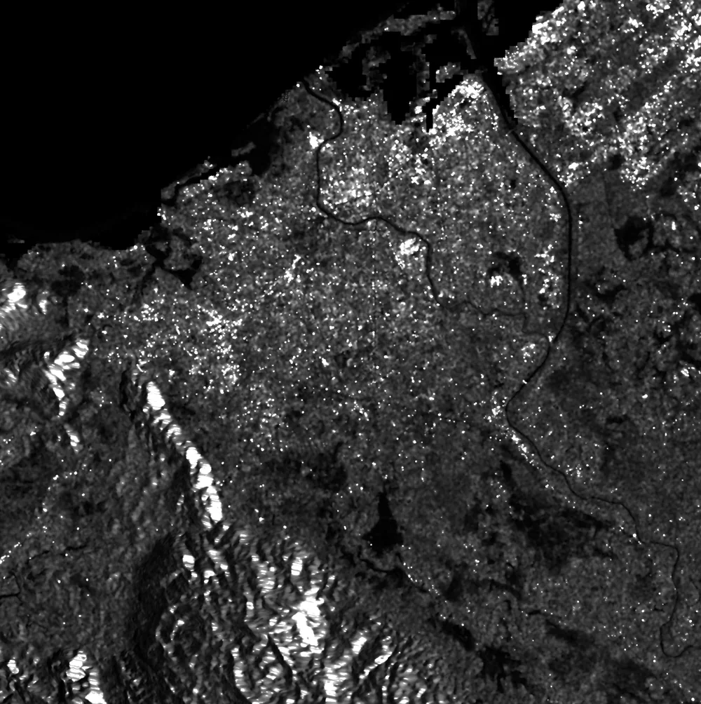
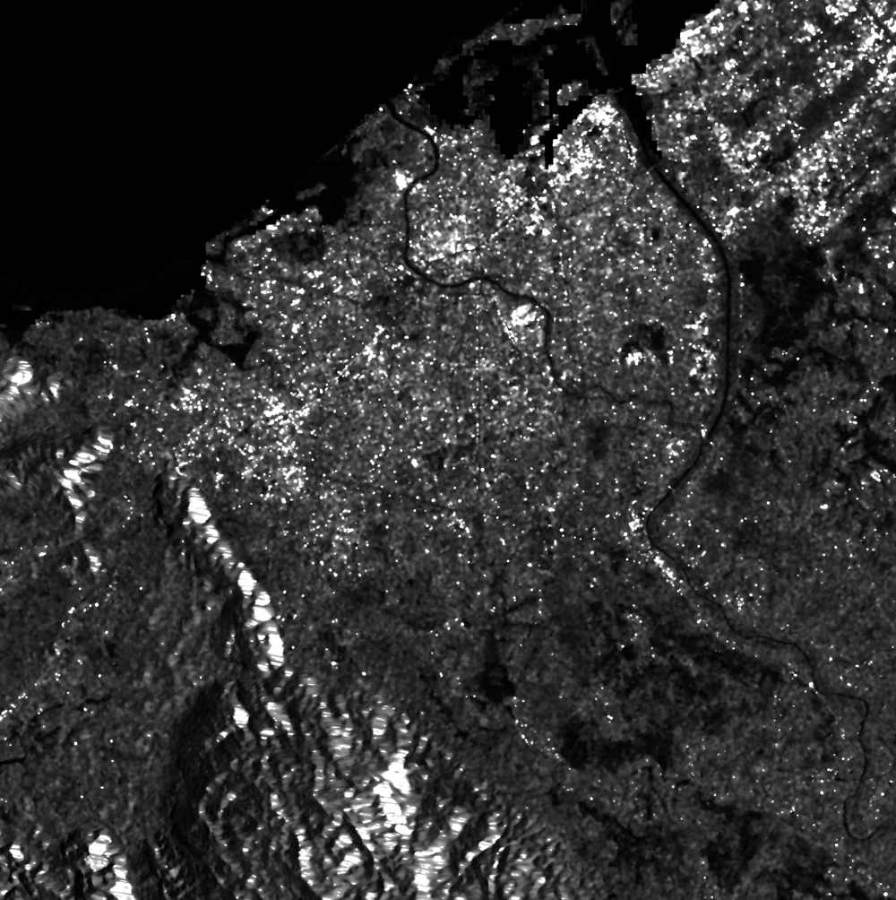
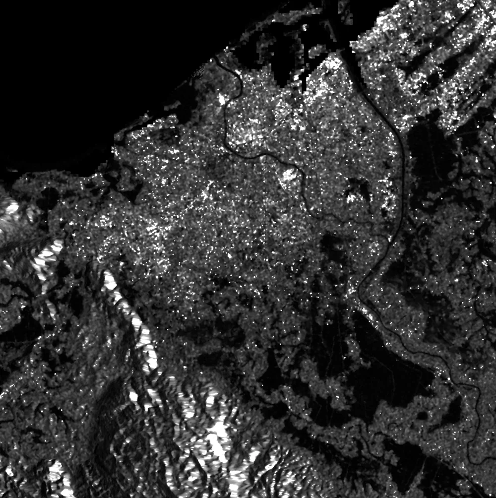
Each tile the model reads is a 224 × 224 px crop of these, stacking all 6 bands (VV + VH at each of the three dates). About 911 such tiles make up the Banda Aceh test split.
04 · Model Training
CS-Mamba U-Net · KuroSiwo dataset · focal+dice loss · 37 epochs
Training loss kept falling after epoch 12, yet that's the checkpoint we kept. Why isn't the lowest-loss model the one you want?
Training source code
# KuroSiwo dataset — download from GitHub / Zenodo
# Patch structure: act/class/hash/{MS1_IVV,MS1_IVH,...,info.json}

from utilities.utilities import prepare_loaders

configs = {
    "task": "segmentation",
    "track": "RandomEvents",
    "train_pickle": "pickle/grid_dict_full.pkl",
    "test_pickle": "pickle/grid_dict_full.pkl",
    # KuroSiwo train/val/test split (European flood events)
    "train_acts": [118, 324, 411, 427],
    "val_acts":   [279, 417, 445],
    "test_acts":  [421, 497, 502],
    # 6-channel input: pre2(VV,VH) + pre1(VV,VH) + post(VV,VH)
    "inputs": ["pre_event_1", "pre_event_2", "post_event"],
    "channels": ["vv", "vh"],
    "clamp_input": 0.15,
    "scale_input": "normalize",
    "data_mean": [0.0953, 0.0264],
    "data_std":  [0.0427, 0.0215],
    "batch_size": 8,
    "num_workers": 4,
    "img_size": 224,
}

train_loader, val_loader, test_loader = prepare_loaders(configs)
print(f"Train: {len(train_loader.dataset)}, Val: {len(val_loader.dataset)}, Test: {len(test_loader.dataset)}")
Train: 6322, Val: 3248, Test: 911
# UNet-style encoder–decoder with Mamba state-space blocks
# 4 scales: 96 → 192 → 384 → 768 channels
# Each block: Conv + 3-direction Mamba scan (H, W, HW-zigzag)

from models.rs_mamba_unet import UNetRSMamba

model = UNetRSMamba(
    in_channels=6,          # VV+VH × 3 dates
    num_classes=3,           # no-water / permanent / flood
    embed_dims=[96, 192, 384, 768],
    depths=[2, 2, 6, 2],      # Mamba blocks per stage
    d_state=16,              # SSM state dimension
    d_conv=4,               # local conv width in Mamba
    expand=2,               # expand ratio
    drop_path_rate=0.1,
)
print(f"Parameters: {sum(p.numel() for p in model.parameters()) / 1e6:.2f}M")
Parameters: 40.55M
import torch

optimizer = torch.optim.AdamW(model.parameters(), lr=1e-4, weight_decay=1e-4)
scaler = torch.cuda.amp.GradScaler()

# Loss: focal (γ=2.5) + dice, weighted 0.35 / 0.65
# Rare classes (permanent water, flood) get upweighted
criterion = FocalDiceLoss(
    focal_gamma=2.5, focal_weight=0.35, dice_weight=0.65,
    class_weights=[0.2, 2.5, 4.0]
)

for epoch in range(37):
    model.train()
    for batch in train_loader:
        image = torch.cat([pre2, pre1, post], dim=1).cuda()  # (B,6,224,224)
        mask = mask.cuda()                                      # (B,224,224)

        with torch.cuda.amp.autocast():
            logits = model(image)                               # (B,3,224,224)
            loss = criterion(logits, mask)

        scaler.scale(loss).backward()
        scaler.step(optimizer)
        scaler.update()
        optimizer.zero_grad()

    # Validate & early-stop on best val mIoU
    val_miou = evaluate(model, val_loader)
    if val_miou > best_val:
        best_val = val_miou
        torch.save(model.state_dict(), "best_checkpoint.pth")
Epoch  0: train_loss=1.842  val_mIoU=0.4123
Epoch  5: train_loss=0.631  val_mIoU=0.6847
Epoch 10: train_loss=0.389  val_mIoU=0.7412
Epoch 12: train_loss=0.342  val_mIoU=0.7598  ★ best checkpoint saved
Epoch 15: train_loss=0.298  val_mIoU=0.7531
Epoch 20: train_loss=0.241  val_mIoU=0.7489
...
Epoch 37: train_loss=0.178  val_mIoU=0.7302  (overfitting)
# Export best checkpoint for deployment (browser / edge / GPU server)
model.load_state_dict(torch.load("best_checkpoint.pth"))
model.eval()

dummy = torch.randn(1, 6, 224, 224)
torch.onnx.export(model, dummy, "cs_mamba_fp16.onnx",
    input_names=["input"], output_names=["logits"],
    dynamic_axes={"input": {0: "batch"}},
    opset_version=17)
Exported cs_mamba_fp16.onnx (82.3 MB, opset 17)
Input:  input  — float32[batch, 6, 224, 224]
Output: logits — float32[batch, 3, 224, 224]
05 · Inference & Interpretation
CS-Mamba · 40.55M params · ONNX WebAssembly · pick a patch · probe with noise & occlusion
Add noise and the mask shifts. Is the model reading water — or just texture? How could you tell the difference?
import onnxruntime as ort

sess = ort.InferenceSession("cs_mamba_fp16.onnx",
    providers=["CUDAExecutionProvider", "CPUExecutionProvider"])

# input: (1, 6, 224, 224) float32
x = np.fromfile("input.bin", dtype=np.float32).reshape(1, 6, 224, 224)
logits = sess.run(None, {"input": x})[0]  # (1, 3, 224, 224)

mask = logits.argmax(axis=1)[0]  # (224, 224) uint8
# 0 = no water, 1 = permanent water, 2 = flood
InferenceSession providers : ['CPUExecutionProvider']   # WebAssembly
input  : float32 (1, 6, 224, 224)
logits : float32 (1, 3, 224, 224)
mask   : uint8   (224, 224)  ∈ {0, 1, 2}
forward pass: 182 ms · deterministic (same input → same mask)import scipy.special prob = scipy.special.softmax(logits, axis=1) # (1, 3, H, W) confidence = prob.max(axis=1)[0] # (H, W) ∈ [0.33, 1.0] # high conf → dark · low conf → amber glow at class boundaries # Perturbation stress-test (the σ / occlude controls below): x_noisy = x + np.random.randn(*x.shape) * sigma x_occ = x.copy(); x_occ[:, :, y0:y1, x0:x1] = 0
confidence = prob.max(1)  →  (224, 224)  ∈ [0.33, 1.00]
mean confidence : 0.86   ·   low-confidence (<0.5) pixels : 7.4%
noise σ = 0.04  →  changed pixels : 2.1%
occlusion box   →  flood-area Δ : −3.8%
↳ try it below — the console runs the same model in your browser
Pick a patch on the scene — its mask + per-class split show here.
06 · Validation
GT comparison · full-AOI panorama · OOD application
CS-Mamba trails on validation but leads on the held-out test events. Which number do you trust — and how is the no-ground-truth case checked at all?
from sklearn.metrics import confusion_matrix

cm = confusion_matrix(gt.flatten(), pred.flatten(), labels=[0,1,2])
for c in range(3):
    tp = cm[c, c]
    iou = tp / (cm[c,:].sum() + cm[:,c].sum() - tp)
    print(f"Class {c}: IoU = {iou:.4f}")
| Class | Recall | Prec. | F1 | IoU |
|---|---|---|---|---|
| No water | 98.3 | 98.0 | 98.1 | 96.4 |
| Permanent | 89.4 | 87.9 | 88.6 | 79.6 |
| Flood | 74.0 | 81.7 | 77.7 | 63.5 |
| Mean | 87.2 | 89.2 | 88.1 | 79.8 |
val mIoU 75.9% → test mIoU 79.8% (+3.8 pp) — generalises, not overfits
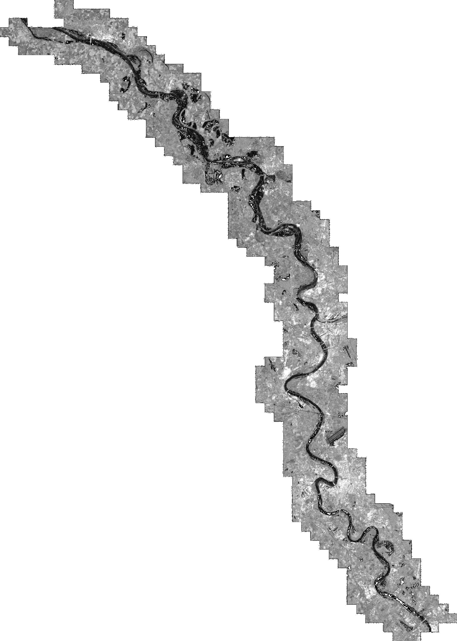
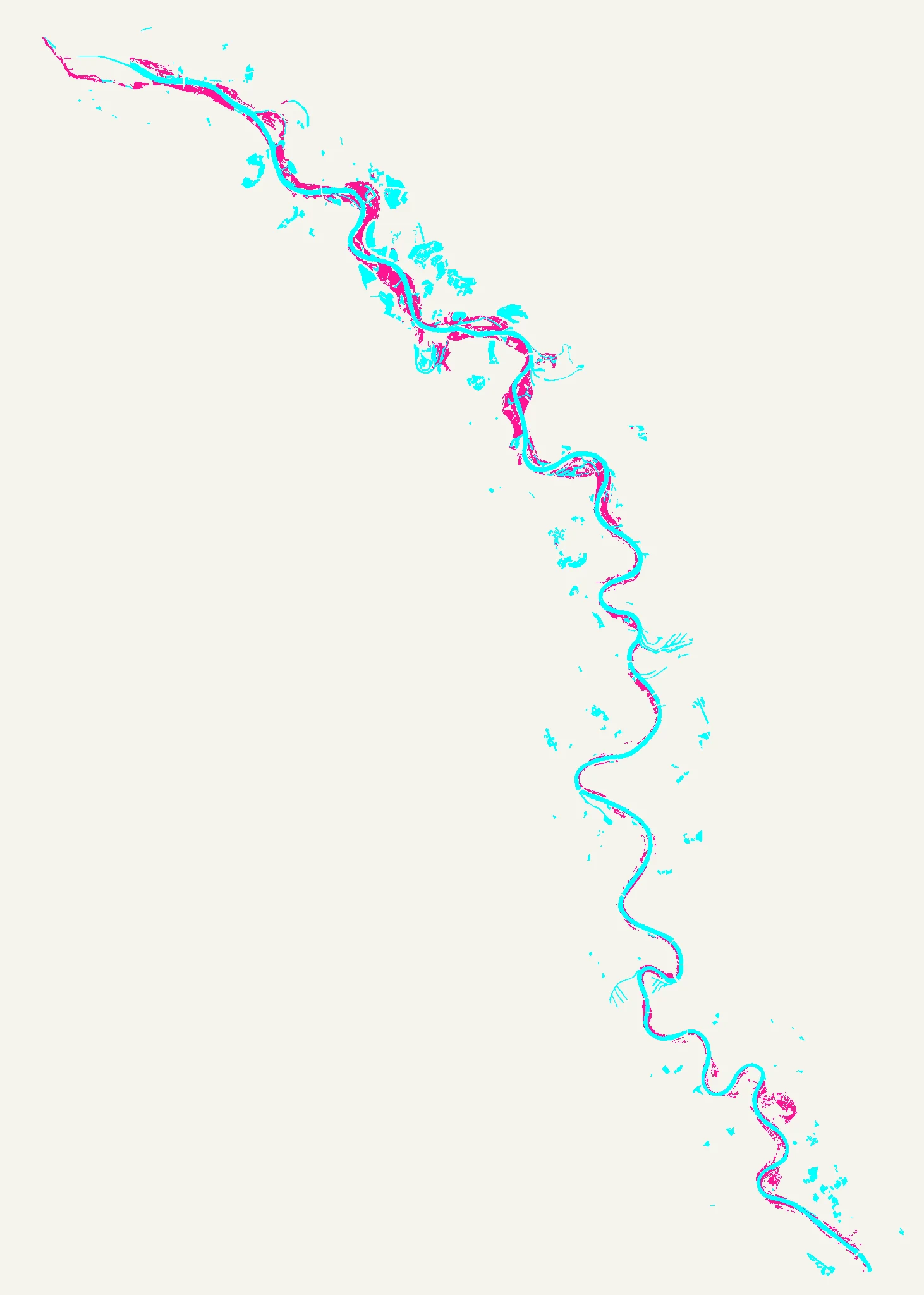
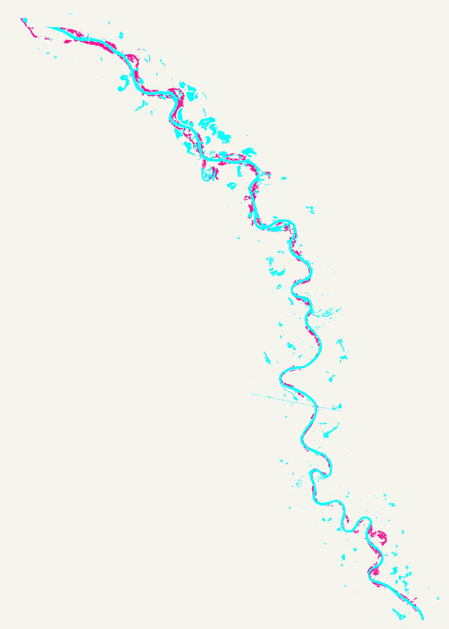
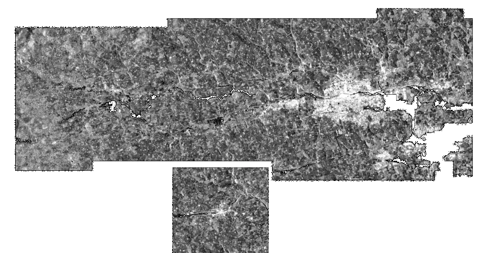
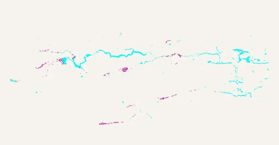
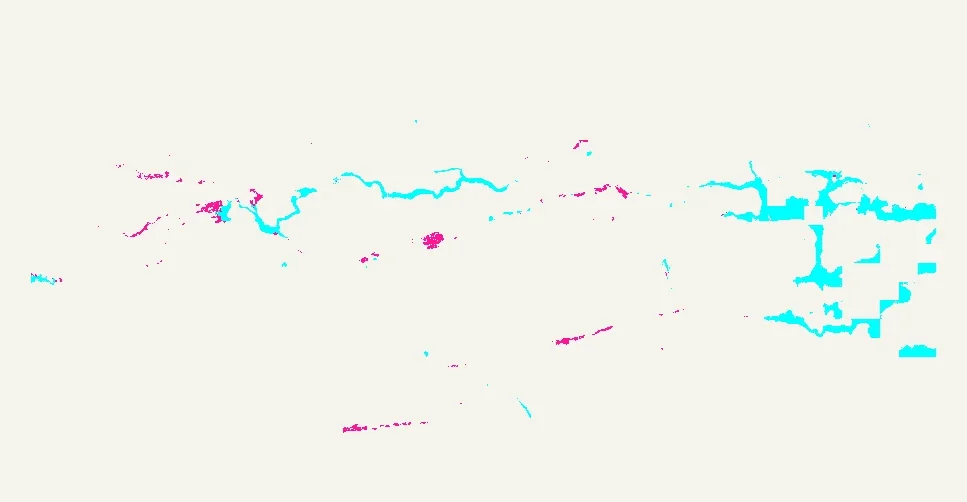
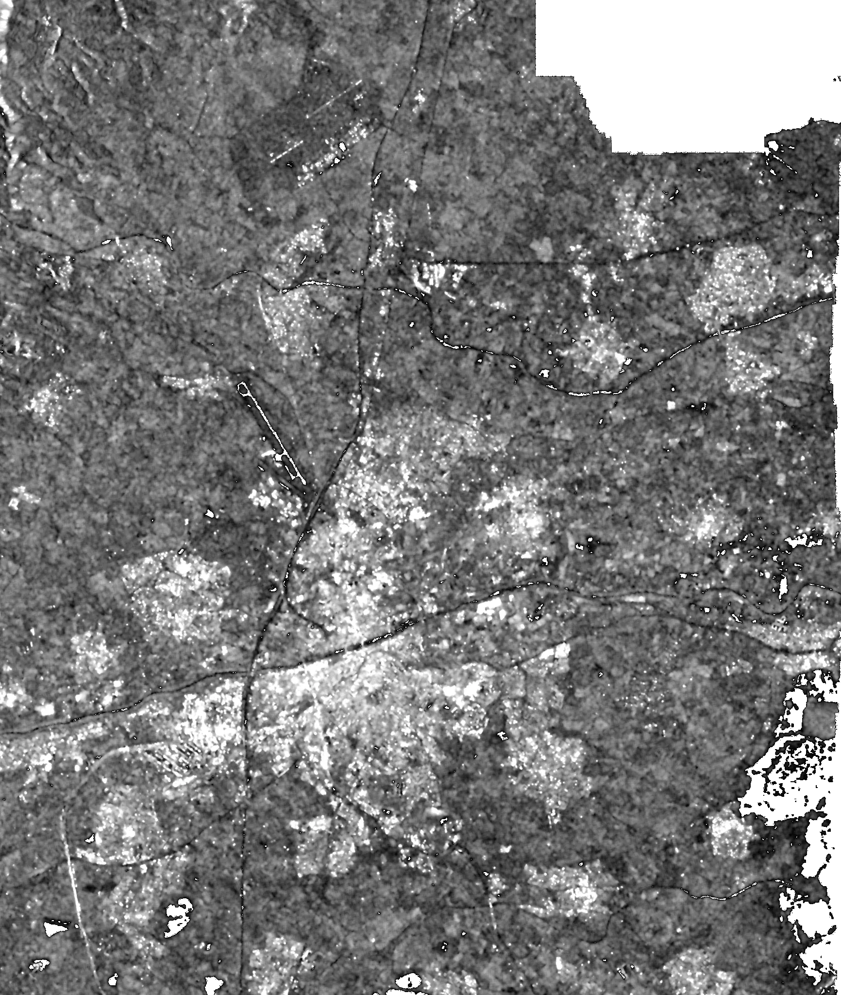
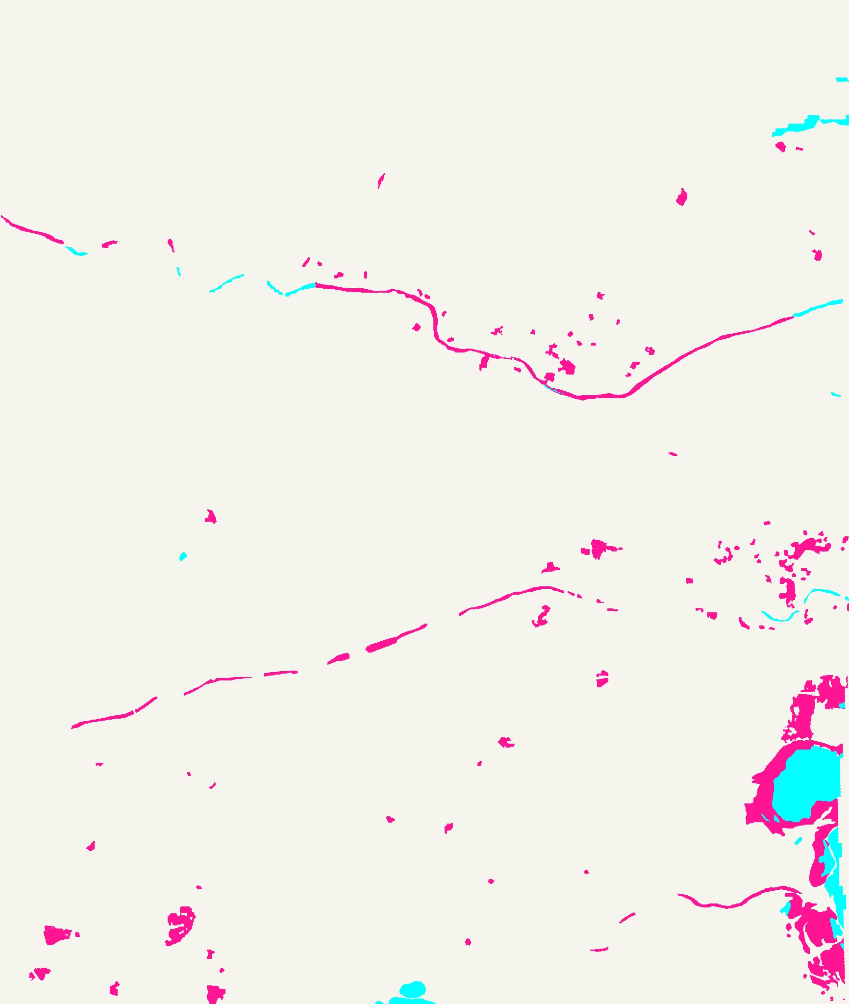
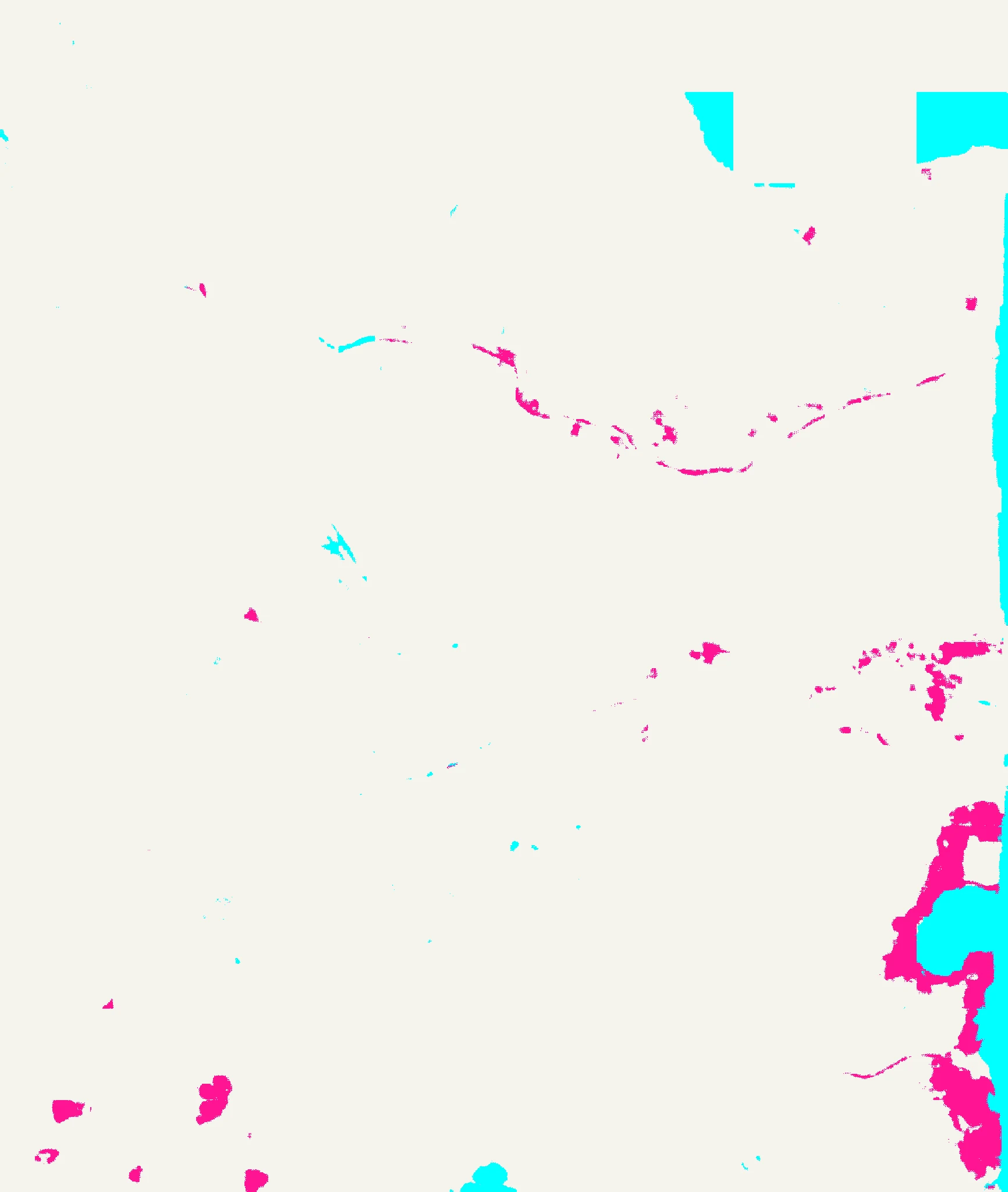
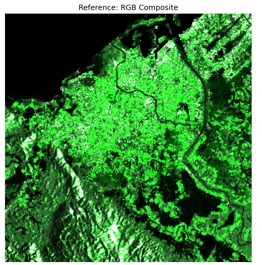
Not a CEMS activation — external OOD validation. Flood occurred months after paper publication.
07 · Bring your own SAR
Judge mode · run your own scene through the deployed model — in your browser, no server
Feed it a shape it never saw in training. Does it truly generalise — or just match the texture it already knows?
dark = smooth water · bright = rough land. Adding noise σ or an occlusion box below degrades these inputs too — watch the SAR get grainy and the mask below respond.
Run your own scene through the deployed model
Everything above ran on our scenes. Now bring your own: drop a normalised input.bin, or six GeoTIFF bands (pre-2 / pre-1 / post × VV+VH) and pick a clamp preset. It preprocesses and runs the same in-browser ONNX — no upload to any server, no ground truth needed. Add noise or drag an occlusion box to probe what the model decided.
Drop your own SAR below — it runs through the exact deployed model and the per-class split appears here.
Upload your own SAR · optional · advanced
Beyond the synthetic test scenes above, bring real data. The model takes a 6-channel, 3-acquisition stack — pre-2 / pre-1 / post, each VV + VH, co-registered at 224×224. Two ways:
D2 · drop an input.bin
The already-normalised tensor we ship per tile (6×224×224 little-endian float32, 1,204,224 bytes). Exact, byte-for-byte reproduction — no preprocessing applied.
D3 · six GeoTIFF bands
One single-band float GeoTIFF per slot (linear σ0). We resample each to 224×224 and apply the model's training-time preprocessing — clamp + per-polarisation standardisation — under the normalization preset you pick below.
clamp 0.15 · VV (μ 0.0953, σ 0.0427) · VH (μ 0.0264, σ 0.0215). For a bright out-of-distribution scene like Banda Aceh, the KuroSiwo training preset misses the flood almost entirely. Switch to a Banda-adapted preset — the recommended one also raises the clamp to 0.30 — to recover it. Each preset re-fits the per-scene statistics and sets the clamp; change it and re-run to watch the effect on your own tile.
Your uploaded tile becomes the live input — the noise slider and occlusion box above then operate on it. Nothing is uploaded to a server; parsing and inference run entirely in your browser.